Elastic Expansion Strategy (Bollinger Bands)
Basic Overview
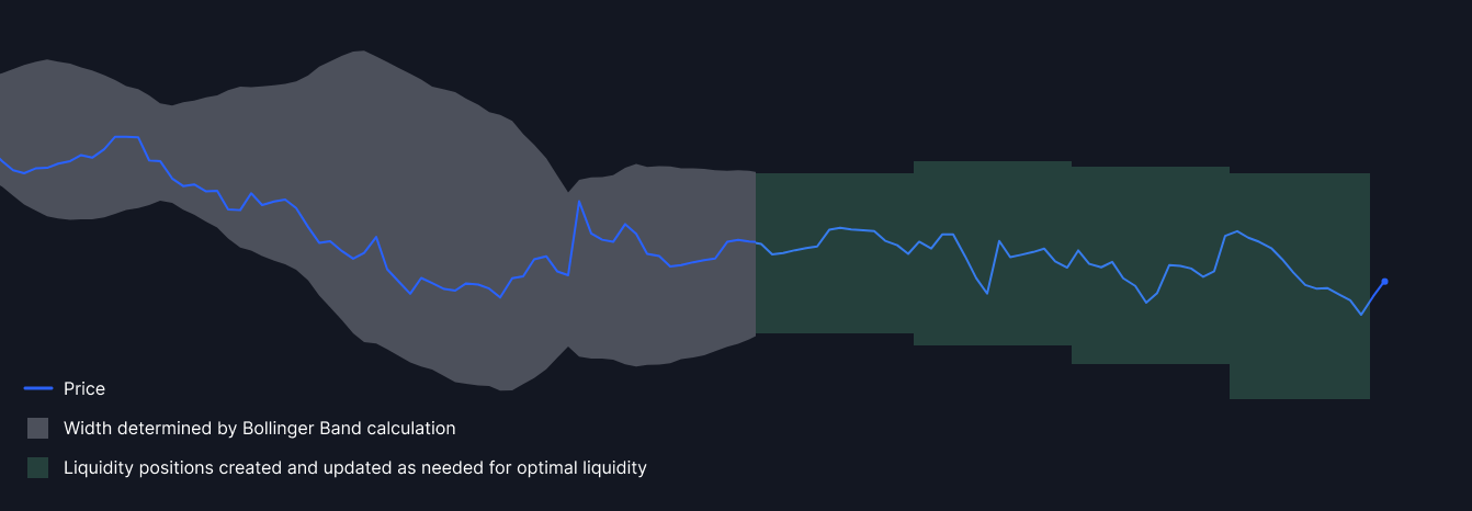
The Elastic Expansion strategy or Bollinger Bands Strategy is an advanced market making approach that uses statistical calculations to identify a range of possible prices for an asset in the next period. By leveraging moving averages and volatility measures, this strategy helps determine the optimal range for liquidity positions, adapting to market conditions and potential price fluctuations.
Ideal Applications

In some instances this strategy can be effective in higher volatitliy token pairings when configured appropriately.
This strategy requires candle data to operate, ensure there is a reliable data source for the candles for proper execution.
Advanced Description and Uses
Strategy Details
The Bollinger Bands Strategy operates by:
- Calculating a simple moving average (SMA) of the asset's price over a specified period
- Determining upper and lower bands based on standard deviations from the SMA
- Using these bands to identify potential overbought or oversold conditions
- Adjusting liquidity positions based on the asset's price relative to the bands
Key Features
- Dynamic Range Calculation
- Volatility-Based Position Sizing
- Adaptive to Market Conditions
- Customizable Parameters
This strategy has rebalance trigger support and liquidity curve support.
Strategic Advantages
- Enhanced Market Sensitivity
- Optimized for Various Volatility Levels
- Potential for Capturing Short-Term Price Movements
- Risk Management through Statistical Boundaries
Technical Explanation
The Bollinger Bands Strategy uses statistical calculations to create a dynamic range for liquidity provision, adapting to market volatility and trends.
Core Mechanics
Bollinger Bands Calculation:
- Middle Band: n-period simple moving average (SMA)
- Upper Band: Middle Band + (k * n-period standard deviation)
- Lower Band: Middle Band - (k * n-period standard deviation)
Where:
- n is the number of periods used for the SMA and standard deviation calculation
- k is the number of standard deviations to be added or subtracted from the middle band
Parameter Configuration:
- Typical values are n = 20 and k = 2
- These can be adjusted based on the asset characteristics and trader preferences
Position Management:
- When price approaches the upper band: Potential overbought condition
- When price approaches the lower band: Potential oversold condition
- Use these signals to adjust liquidity positions accordingly
Liquidity Provision Strategy:
- Concentrate liquidity within the bands
- Adjust position sizes based on proximity to band edges
- Consider reducing exposure when price moves beyond the bands
Implementation Considerations
- Regular recalculation of bands is necessary to adapt to changing market conditions
- The strategy's effectiveness can vary depending on market trends and volatility
- Combining with other indicators or strategies may enhance performance
- Backtesting with different parameter values is recommended for optimization
Future Enhancements
- Ongoing normalization feature updates may lead to further refinements
- Potential for integration with other statistical or machine learning approaches
Similar Use Cases
Many use cases for this strategy are similar to the Moving Volatility Strategy, including:
- Adapting to varying levels of market volatility
- Optimizing liquidity provision in trending markets
- Managing risk in assets prone to price fluctuations
By leveraging statistical measures to create dynamic liquidity provision ranges, the Bollinger Bands Strategy offers liquidity providers a sophisticated tool for adapting to market conditions, optimizing positions, and managing risk across various asset types and market scenarios.